3D Wing shape optimization via Reinforcement Learning

This example wiill show how to train an agent that optimizes wings.

Define operating conditions

from pyLOM.RL import (
    create_env,
    WingOperatingConditions,
    WingParameterizerConfig,
    AerosandboxWingSolver,
)

from stable_baselines3 import PPO

import torch

# training should be faster with single thread
torch.set_num_threads(1)

operating_conditions = WingOperatingConditions(
    alpha=2.0,
    altitude=500,
    velocity=200,
)

Shape parameterization and design space

To parametrize the wing secntions and regions need to be defined. Each secion is defined by its chord length, an airfoil and a twist. Each region is defined by its lenght (span) and the 2 angles formed by the secions (sweep and diherdal). Note that there must be one more section than regions.

Similar to the 2D case, we can use AirfoilCSTParametrizer directly or AirfoilParameterizerConfig, that will create an instance of AirfoilCSTParametrizer with some default parameters

parameterizer = WingParameterizerConfig().create_parameterizer()

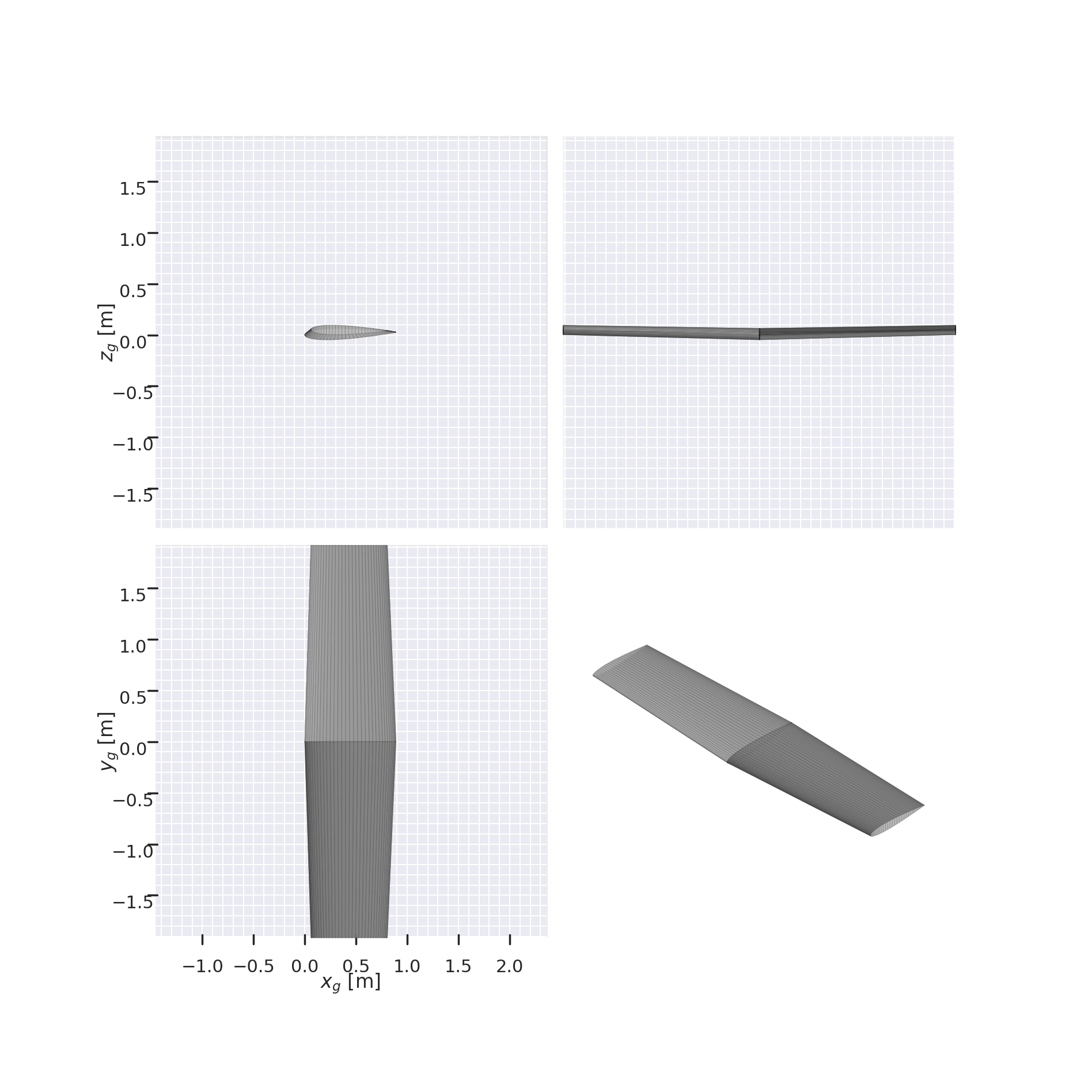
Here is an example of how a wing can be created from its parameters using the parameterizer. Note that since the default parameterizer has only 2 sections and 1 region, the parameters must have exactly 2 sections and 1 region, otherwise it will not work. To use more secions, other parameterizer defined for more sections would be required

chords = [0.8, 0.6]
twists = [0.1, 0.2]
spans = [2.0]
sweeps = [5]
diheds = [5]

wing_params = chords + twists + spans + sweeps + diheds

wing = parameterizer.get_shape_from_params(wing_params)
wing.draw_three_view()

array([[<Axes3D: zlabel='$z_g$ [m]'>, <Axes3D: >],
       [<Axes3D: xlabel='$x_g$ [m]', ylabel='$y_g$ [m]'>, <Axes3D: >]],
      dtype=object)

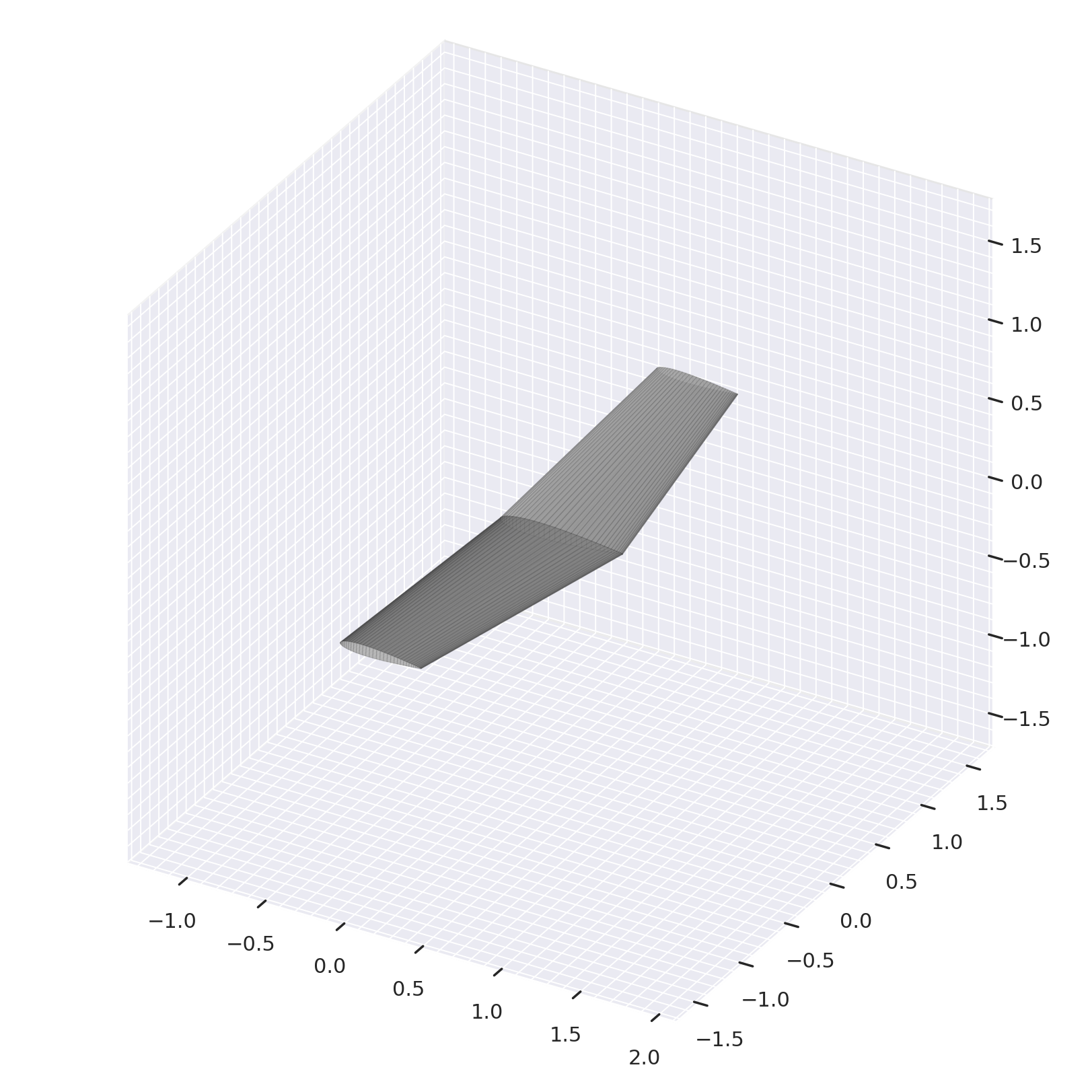
We can generate too a random wing within the desing parameters bounds

random_wing_params = parameterizer.generate_random_params()
wing = parameterizer.get_shape_from_params(random_wing_params)
wing.draw_three_view()

array([[<Axes3D: zlabel='$z_g$ [m]'>, <Axes3D: >],
       [<Axes3D: xlabel='$x_g$ [m]', ylabel='$y_g$ [m]'>, <Axes3D: >]],
      dtype=object)

Define the solver

As in the airfoil example, a solver is needed. In this case the 3D solver integrated in aerosandbos will be used

solver = AerosandboxWingSolver(
    alpha=operating_conditions.alpha,
    atmosphere=operating_conditions.atmosphere, # this is created automatically when the altitude is defined
    velocity=operating_conditions.velocity,
)

Create the environment

The enviroment can be created either with gym.make or with create_env. For this example parallel environment will be used to speed up the training, so create_env will be easier to use.

# env = gym.make(
#     "ShapeOptimizationEnv-v0",
#     solver=solver,
#     parameterizer=parameterizer,
#     episode_max_length=64,
# )
NUM_ENVS = 8
env = create_env(
    "aerosandbox",
    operating_conditions=operating_conditions,
    episode_max_length=64,
    parameterizer=parameterizer,
    num_envs=NUM_ENVS,
)

Define the PPO agent and train it on the environment

We define the hyperparameters here to train an agent. Since parallel environments are used, n_steps, which indicates after how many steps the weights of the agent are updated, needs to be divided by the number of environments

ppo_parameters = {
    'learning_rate': 2.5e-4,
    'n_steps': 2048 // NUM_ENVS,
    'batch_size': 32,
    'n_epochs': 20,
    'gamma': 0.3,
    'gae_lambda': 0.95,
    'clip_range': 0.4,
    'ent_coef': 0.005,
    'verbose': 1,
    'policy_kwargs': {'net_arch': dict(pi=[256, 256], vf=[256, 256])},
}
training_timesteps = 15000

model = PPO("MlpPolicy", env, **ppo_parameters)

Using cpu device

model.learn(total_timesteps=training_timesteps)
model.save("wing_agent")

If you want to use a model that is already trained you can load it

model = PPO.load("wing_agent")

Test the agent

Evaluation for the 3D optimization is easier because we can evaluate the agent with the random resets of the environment. Thus, the built-it fucntion evaluate_policy from stable baselines 3 can be used

from pyLOM.RL import (
    run_episode,
)
from stable_baselines3.common.evaluation import evaluate_policy

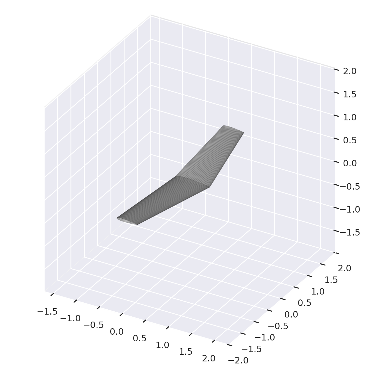
First, an eval_env is defined without parallelization. Then an initial wing is randomly generated, but note that any abs.Wing within the bounds of the parameterizer can be optimized

eval_env = create_env(
    "aerosandbox",
    operating_conditions=operating_conditions,
    episode_max_length=64,
    parameterizer=parameterizer,
    num_envs=1,
)
obs, info = eval_env.reset()
initial_wing = info['shape']
initial_wing.draw(backend="matplotlib")

/home/david/miniconda/envs/pylom-rl/lib/python3.11/site-packages/gymnasium/spaces/box.py:235: UserWarning: WARN: Box low's precision lowered by casting to float32, current low.dtype=float64
  gym.logger.warn(
/home/david/miniconda/envs/pylom-rl/lib/python3.11/site-packages/gymnasium/spaces/box.py:305: UserWarning: WARN: Box high's precision lowered by casting to float32, current high.dtype=float64
  gym.logger.warn(
/home/david/miniconda/envs/pylom-rl/lib/python3.11/site-packages/gymnasium/utils/passive_env_checker.py:134: UserWarning: WARN: The obs returned by the `reset()` method was expecting numpy array dtype to be float32, actual type: float64
  logger.warn(
/home/david/miniconda/envs/pylom-rl/lib/python3.11/site-packages/gymnasium/utils/passive_env_checker.py:158: UserWarning: WARN: The obs returned by the `reset()` method is not within the observation space.
  logger.warn(f"{pre} is not within the observation space.")

mean_reward, std_reward = evaluate_policy(model, eval_env, n_eval_episodes=20, warn=False)

print(f"Mean CL/CD improvement: {mean_reward:.2f} +/- {std_reward:.2f}")

Mean CL/CD improvement: 7.38 +/- 4.30

rewards, states = run_episode(model, eval_env, initial_shape=initial_wing)
eval_env.render()

(None, Wing 'Main Wing' (2 xsecs, symmetric))

States contains the parameters of the wings, but if we want to visualize them we need asb.Wing objects. Similar to the airfoil example, we can convert them with the parameterizer

wings = list(map(lambda x: parameterizer.get_shape_from_params(x), states))

Now any intermediate wing of the optimization can be visualized. A similar animation to the airfoil example of the optimization process is available too, but for that you will need to install manim with conda install -c conda-forge manim.

If the video generation takes too long you can adjust the quality changing the “-qp” option:

* -ql: for low quality * -qm: for medium quality * -qh: for high quality * -qp: for production quality (the highest)

from pyLOM.RL import WingEvolutionAnimation
from manim import *

%%manim -qp -v WARNING WingEvolutionAnimation

WingEvolutionAnimation.wings = wings
WingEvolutionAnimation.rewards = rewards
WingEvolutionAnimation.run_time_per_update = 0.1

This is a small trick to actually show the resulting video on the documentation, the code here is not relevant since the previous cell must have already shown it

import base64
from IPython.display import HTML
video_path = "./media/videos/notebook_examples/1440p60/_WingEvolution.mp4"

with open(video_path, "rb") as f:
    video_data = base64.b64encode(f.read()).decode()

HTML(f"""
<video width="800" controls>
    <source src="data:video/mp4;base64,{video_data}" type="video/mp4">
    Your browser does not support the video tag.
</video>
""")